what is non-stationary signals

stationary signals

Hi Friends,

i need to know what is the non stationary signals?

if someone can help me by equations and drawing please....

what is nonstationery

hi Friend,
stationary signals are independent of time eg x[n]=5 DC signal

non-stationary signals are dependent on time x[n] = n ramp signal

Are u asking abt statonary procecess


Happy learning

thank you rramya, as i tolled you. You are very expert.

this is very clear for me.

Added after 3 hours 26 minutes:

Hi rramya,

I am so sorry as i think your answer is not correct. I found out in the following link the answer as followes:

**broken link removed**

Let's take a closer look at this stationarity concept more closely, since it is of paramount importance in signal analysis. Signals whose frequency content do not change in time are called stationary signals . In other words, the frequency content of stationary signals do not change in time. In this case, one does not need to know at what times frequency components exist , since all frequency components exist at all times !!! .

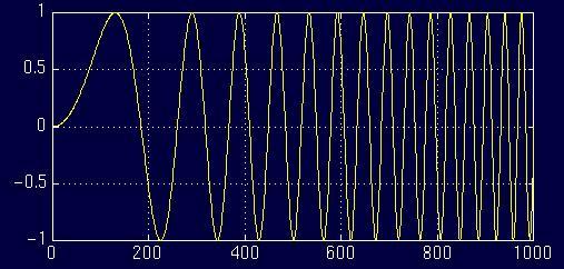
For example the following signal

x(t)=cos(2*pi*10*t)+cos(2*pi*25*t)+cos(2*pi*50*t)+cos(2*pi*100*t)

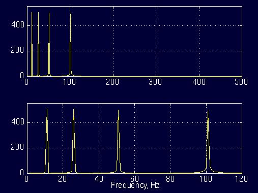
is a stationary signal, because it has frequencies of 10, 25, 50, and 100 Hz at any given time instant. This signal is plotted below:


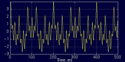
Figure 1.5

And the following is its FT:


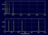
Figure 1.6

The top plot in Figure 1.6 is the (half of the symmetric) frequency spectrum of the signal in Figure 1.5. The bottom plot is the zoomed version of the top plot, showing only the range of frequencies that are of interest to us. Note the four spectral components corresponding to the frequencies 10, 25, 50 and 100 Hz.

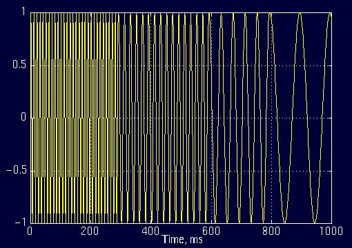
Contrary to the signal in Figure 1.5, the following signal is not stationary. Figure 1.7 plots a signal whose frequency constantly changes in time. This signal is known as the "chirp" signal. This is a non-stationary signal.


Figure 1.7

Let's look at another example. Figure 1.8 plots a signal with four different frequency components at four different time intervals, hence a non-stationary signal. The interval 0 to 300 ms has a 100 Hz sinusoid, the interval 300 to 600 ms has a 50 Hz sinusoid, the interval 600 to 800 ms has a 25 Hz sinusoid, and finally the interval 800 to 1000 ms has a 10 Hz sinusoid.


Figure 1.8

If it is incorrect, please rectify me.

thanks